Exploring African Internet
Exploring NDT & Paris-Traceroute in Africa
This Jupyter notebook visualizes M-Lab test data in Africa. Using BigQuery, we select NDT or paris-traceroute data from clients in Africa. Then, using a world map from Natural Earth and the GeoDataFrame Python packages, we plot the African data using geolocation hints from the data.
This notebook may be downloaded from the GitHub repository for the M-Lab website.
Setup
To do this, we need to install and configure some local dependencies first.
- Install Jupyter
- Install gcloud SDK
- Setup gcloud SDK
# Authenticate your account.gcloud auth login
# Set application default credentials.gcloud auth application-default login
# Set default project.gcloud config set project measurement-lab- Install google-cloud-bigquery package:
pip install --upgrade google-cloud-bigquery- Install GeoPandas and dependencies
pip install geopandas PySAL descartes- Start Jupyter
jupyter-notebookReferences
- Matplotlib - https://matplotlib.org/contents.html
- Pandas - https://pandas.pydata.org/pandas-docs/stable/api.html
- BigQuery - https://cloud.google.com/bigquery/docs/reference/standard-sql/functions-and-operators
- GeoPandas - http://geopandas.org/index.html
%matplotlib inlineimport os
import matplotlib.pyplot as pltimport pandas as pdimport geopandas as gpdimport collectionsimport urllib2import jsonfrom shapely import geometry
# Ignore warnings from various packages.import warningswarnings.filterwarnings("ignore")
# Set project explicitly in the environment to suppress some warnings.os.environ["GOOGLE_CLOUD_PROJECT"] = "measurement-lab"
# Load M-Lab site metadata including site latitude & longitude.mlab_sites_url = 'https://storage.googleapis.com/operator-mlab-oti/metadata/v0/current/mlab-site-stats.json'
# Load the Natural Earth country shapes file.worldmap_url = 'https://d2ad6b4ur7yvpq.cloudfront.net/naturalearth-3.3.0/ne_50m_admin_0_countries.geojson'
# Short list of metros in Africa, for convenience.african_metros = ['tun', 'jnb', 'cpt', 'mpm', 'tnr', 'los', 'nbo', 'acc']
# Number of colors to use when coloring maps.colors = 10
# Default figure size. W x H.figsize = (16, 10)
# Depends on: pip install --upgrade google-cloud-bigqueryfrom google.cloud import bigquery
def run_query(query, project='measurement-lab'): client = bigquery.Client(project=project) job = client.query(query)
results = collections.defaultdict(list) for row in job.result(timeout=600): for key in row.keys(): results[key].append(row.get(key))
return pd.DataFrame(results)# Load shape data.globe_raw = gpd.read_file(worldmap_url)
# Select the global information (except Antarctica).globe = globe_raw[['iso_a2', 'continent', 'geometry']].to_crs('+proj=longlat')globe = globe[globe.continent != 'Antarctica']# Add a new column with a default value of zero to show countries without data.globe['default'] = 0
# Select only Africa.africa = globe[globe.continent == 'Africa'].copy()africa['default'] = 0africa.sample(5)| iso_a2 | continent | geometry | default | |
|---|---|---|---|---|
| 124 | LY | Africa | POLYGON ((25.15048828125001 31.65498046875, 25... | 0 |
| 49 | CV | Africa | (POLYGON ((-24.30825195312497 14.8562988281249... | 0 |
| 142 | ML | Africa | POLYGON ((4.227636718750006 19.1427734375, 4.2... | 0 |
| 239 | ZM | Africa | POLYGON ((32.919921875 -9.407421875000011, 32.... | 0 |
| 223 | UG | Africa | POLYGON ((33.90322265625002 -1.002050781250006... | 0 |
NDT in Africa
How many NDT tests are clients in Africa running to M-Lab servers?
By default, the M-Lab naming service directs clients to the geographically closest M-Lab server. The idea is to use geographic proximity as a proxy for network proximity. So, we expect to see more tests near M-Lab servers.
For a given day, the query below counts all tests from clients in Africa. At the same time we calculate the average download rate per country for all clients.
rates_df = run_query("""SELECT  connection_spec.client_geolocation.country_name as country_name,  connection_spec.client_geolocation.country_code as country_code,  COUNT(*) as count,  AVG(8 * (web100_log_entry.snap.HCThruOctetsAcked /      (web100_log_entry.snap.SndLimTimeRwin +       web100_log_entry.snap.SndLimTimeCwnd +       web100_log_entry.snap.SndLimTimeSnd))) AS download_Mbps
FROM  `measurement-lab.ndt.base`WHERE      TIMESTAMP_TRUNC(log_time, DAY) = TIMESTAMP("2018-11-16")  AND connection_spec.client_geolocation.continent_code = "AF"
  AND connection_spec.data_direction = 1  AND web100_log_entry.snap.HCThruOctetsAcked >= 8192  AND (web100_log_entry.snap.SndLimTimeRwin +    web100_log_entry.snap.SndLimTimeCwnd +    web100_log_entry.snap.SndLimTimeSnd) >= 9000000  AND (web100_log_entry.snap.SndLimTimeRwin +    web100_log_entry.snap.SndLimTimeCwnd +    web100_log_entry.snap.SndLimTimeSnd) < 600000000  AND web100_log_entry.snap.CongSignals > 0  AND (web100_log_entry.snap.State = 1 OR    (web100_log_entry.snap.State >= 5 AND    web100_log_entry.snap.State <= 11))
GROUP BY  country_code, country_name
HAVING  count > 100
ORDER BY country_name, country_code, count desc""")
# Now `rates_df` contains all results from the BigQuery results in the form of a Pandas DataFrame.rates_df.sample(5)| count | country_code | country_name | download_Mbps | |
|---|---|---|---|---|
| 0 | 385 | DZ | Algeria | 1.787968 |
| 1 | 481 | EG | Egypt | 1.942897 |
| 5 | 3001 | MA | Morocco | 5.918805 |
| 10 | 217 | UG | Uganda | 2.270746 |
| 7 | 12824 | ZA | South Africa | 9.959014 |
# Merge the africa dataframe with the rates_df using the 2-letter country codes in both.rates_merged = africa.merge(rates_df, left_on='iso_a2', right_on='country_code')rates_merged.sample(5)| iso_a2 | continent | geometry | default | count | country_code | country_name | download_Mbps | |
|---|---|---|---|---|---|---|---|---|
| 1 | EG | Africa | POLYGON ((34.19814453125002 31.322607421875, 3... | 0 | 481 | EG | Egypt | 1.942897 |
| 4 | MA | Africa | POLYGON ((-4.628320312499966 35.20639648437501... | 0 | 3001 | MA | Morocco | 5.918805 |
| 3 | KE | Africa | (POLYGON ((40.99443359375002 -2.15839843749998... | 0 | 1702 | KE | Kenya | 5.796839 |
| 8 | TZ | Africa | (POLYGON ((39.711328125 -7.977441406250024, 39... | 0 | 120 | TZ | Tanzania | 1.249333 |
| 10 | ZA | Africa | (POLYGON ((37.85693359375003 -46.9442382812499... | 0 | 12824 | ZA | South Africa | 9.959014 |
Test Counts
# First, plot the plain African map with all countries represented.ax0 = africa.plot(column='default', color='white', edgecolor='lightgrey', figsize=figsize)# Next, plot the merged rates dataframe on top of the base map. Only countries with data will be shown._ = rates_merged.plot(ax=ax0, column='count', cmap='Blues', scheme='Fisher_Jenks', k=colors, legend=True, legend_kwds={"loc": 3}, edgecolor='lightgrey')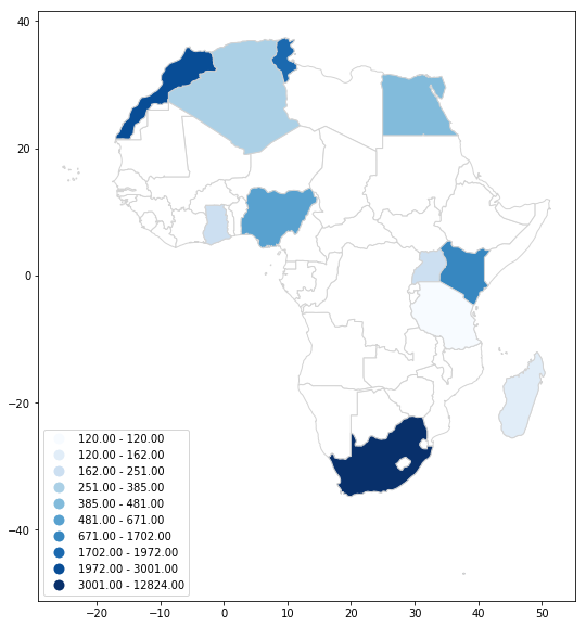
M-Lab Metro Locations
While the map above highlights countries where users are running NDT tests, it does not reveal the location of M-Lab servers used to run those tests.
To add M-Lab server locations to the map, next we will load the M-Lab site configuration for Africa.
# Download the M-Lab site configuration.response = urllib2.urlopen(mlab_sites_url)sites = json.loads(response.read())
# Collect all sites in Africa, creating a geometry.Point for each one.all_map = {}africa_map = {}for row in sites:    metro = row['site'][0:3]    all_map[metro] = (metro, geometry.Point(row['longitude'], row['latitude']))    if metro in african_metros:        africa_map[metro] = all_map[metro]
# Convert the dict into a GeoDataFrame.all_locations = gpd.GeoDataFrame(pd.DataFrame.from_dict(    all_map, orient='index', columns=['metro', 'location']), geometry='location')africa_locations = gpd.GeoDataFrame(pd.DataFrame.from_dict(    africa_map, orient='index', columns=['metro', 'location']), geometry='location')
print africa_locations.keys()Index([u'metro', u'location'], dtype='object')Test Counts With M-Lab Metro Locations
# Repeat the steps for plotting Africa test counts.ax0 = africa.plot(column='default', color='white', edgecolor='lightgrey', figsize=figsize)ax1 = rates_merged.plot(ax=ax0, column='count', cmap='Blues', scheme='Fisher_Jenks', k=colors, legend=True, legend_kwds={"loc": 3}, edgecolor='lightgrey')# Add the M-Lab metro locations.africa_locations.plot(ax=ax1, color='red', markersize=20)_ = ax1.set_title('NDT Test Counts and M-Lab Metro Locations')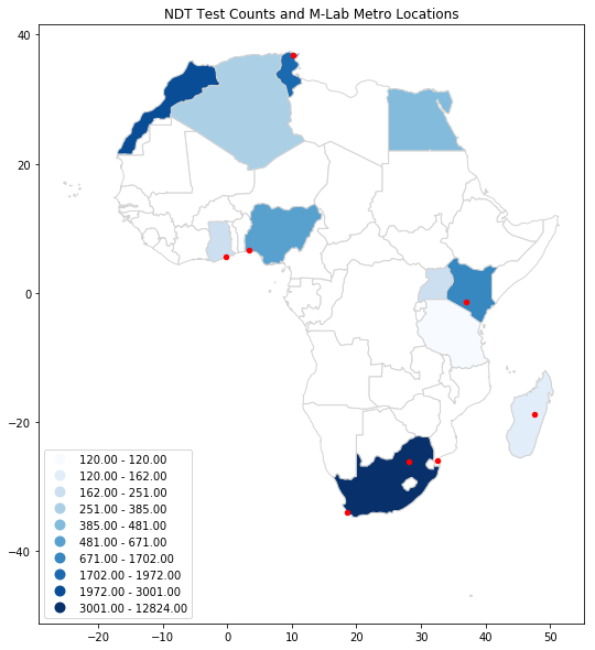
NDT Test Rates
f, ax = plt.subplots(1, 2, figsize=figsize)
ax0 = africa.plot(ax=ax[0], column='default', color='white', edgecolor='lightgrey', figsize=figsize)ax1 = rates_merged.plot(ax=ax0, column='count', cmap='Blues', scheme='Fisher_Jenks',                        k=colors, legend=True, legend_kwds={"loc": 3}, edgecolor='lightgrey')africa_locations.plot(ax=ax1, color='red', markersize=20)
ax0 = africa.plot(ax=ax[1], column='default', color='white', edgecolor='lightgrey', figsize=figsize)ax2 = rates_merged.plot(ax=ax0, column='download_Mbps', cmap='Greens', scheme='Fisher_Jenks',                        k=colors, legend=True, legend_kwds={"loc": 3}, edgecolor='lightgrey')africa_locations.plot(ax=ax2, color='red', markersize=20)
_ = ax1.set_title('Test Counts')_ = ax2.set_title('Download Rates (Mbps)')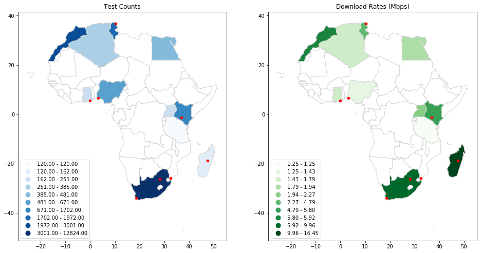
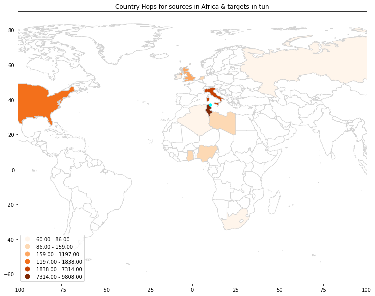
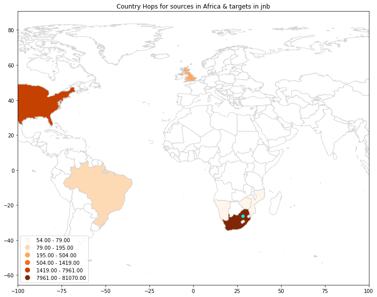
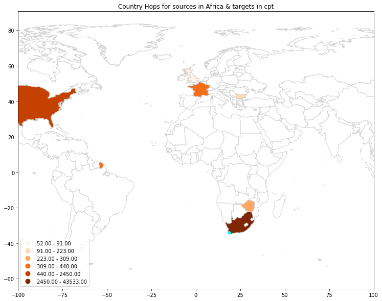
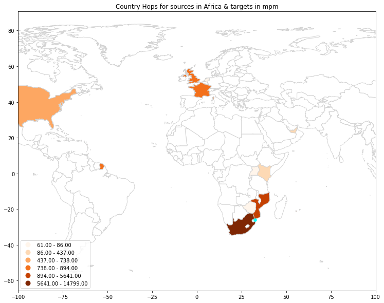
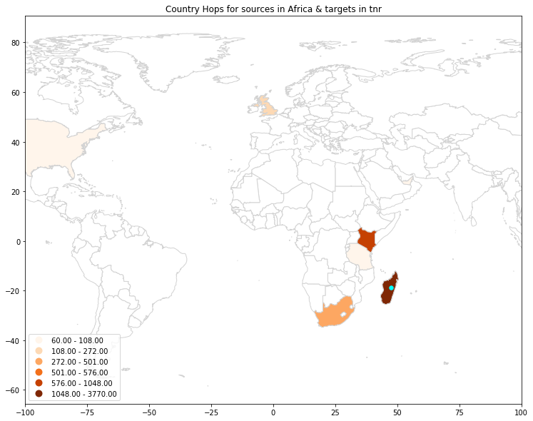
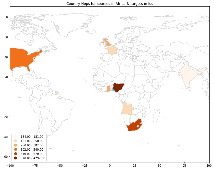
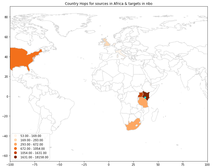
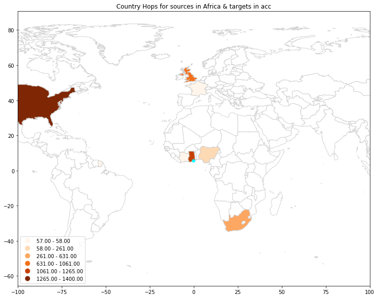
Paris-Traceroute in Africa
How are clients in Africa routed to M-Lab servers?
Every time a client machine contacts and M-Lab server, the server starts a paris-traceroute from the M-lab server to the client remote IP. Each paris-traceroute hop is annotated with geo-location metadata for the intermediate router IP address, including the country.
For a given day, the query below counts the hops in all countries visited between all clients in Africa and the African M-Lab server they contacted. The query is limited to NDT tests (ports 3010 and 3001).
df_hops = {}for metro in african_metros:    print metro,    df_hops[metro] = run_query("""SELECT  paris_traceroute_hop.dest_geolocation.country_code as dest_country_code,  COUNT(*) as hops
FROM  `measurement-lab.traceroute.base`
WHERE      TIMESTAMP_TRUNC(log_time, DAY) = TIMESTAMP("2018-11-16")  AND REGEXP_CONTAINS(test_id, r"mlab[1-4].%s\d\d")  AND connection_spec.client_geolocation.continent_code = "AF"  AND (REGEXP_CONTAINS(test_id, ".*3010.paris.gz") OR REGEXP_CONTAINS(test_id, ".*3001.paris.gz"))
GROUP BY  dest_country_code
HAVING  hops > 50
ORDER BY  hops desc""" % metro)
tun jnb cpt mpm tnr los nbo accfor metro in african_metros: if not len(df_hops[metro]): print "Skipping %s" % metro continue
hops_merged = globe.merge(df_hops[metro], left_on='iso_a2', right_on='dest_country_code')
ax1 = globe.plot(column='default', color='white', edgecolor='lightgrey', figsize=figsize) ax2 = hops_merged.plot(ax=ax1, column='hops', cmap='Oranges', scheme='Fisher_Jenks', k=6, legend=True, legend_kwds={"loc": 3}, edgecolor='lightgrey') ax2.set_title('Country Hops for sources in Africa & targets in %s' % metro) africa_locations[africa_locations.metro == metro].plot(ax=ax2, color='cyan', markersize=30) ax2.set_xbound(-100, 100)